Table of Contents
In this tutorial, we use a subset of the bulk RNAseq data of prostate adenocarcinoma (PRAD) from TCGA (https://portal.gdc.cancer.gov/) as an example to demonstrate how to run DeMixT. The analysis pipeline consists of the following steps:
- Obtaining raw read counts for the tumor and normal RNAseq data
- Loading libraries and data
- Data preprocessing
- Deconvolution using DeMixT
1. Obtain raw read counts for the tumor and normal RNAseq data
The raw read counts for the tumor and normal samples from TCGA PRAD are downloaded from TCGA data portal. One can also generate the raw read counts from fastq or bam files by following the GDC mRNA Analysis Pipeline.
2. Load libraries and data
2.1 Load library
library(DeMixT)
library(psych)
2.2 Load input data
load("./docs/etc/PRAD.RData")
Three data are included in the PRAD.RData file.
PRAD: Read counts matrix (gene x sample) with genes as row names and sample ids as column names.Normal.id: TCGA ids of PRAD normal samples.Tumor.idTCGA ids of PRAD tumor samples.
A glimpse of PRAD:
head(PRAD[,1:5])
cat('Number of genes: ', dim(PRAD)[1], '\n')
cat('Number of normal sample: ', length(Normal.id), '\n')
cat('Number of tumor sample: ', length(Tumor.id), '\n')

         TCGA-CH-5761-11A TCGA-CH-5767-11B TCGA-EJ-7115-11A TCGA-EJ-7123-11A TCGA-EJ-7125-11A
TSPAN6               3876             7095             5542             2747             8465
TNMD                   14               51               13               24               63
DPM1                 1162             2665             1544             1974             2984
SCYL3                 777             1517             1096             1231             1514
C1orf112              136              343              214              280              339
FGR                   230              511              263              755              262
Number of genes:  59427
Number of normal sample:  20
Number of tumor sample:  30
3. Data preprocessing
Conduct data cleaning and normalization before running DeMixT.
PRAD = PRAD[, c(Normal.id, Tumor.id)]
selected.genes = 9000
cutoff_normal_range = c(0.1, 1.0)
cutoff_tumor_range = c(0, 2.5)
cutoff_step = 0.1

preprocessed_data = DeMixT_preprocessing(PRAD,
                                         Normal.id,
                                         Tumor.id,
                                         selected.genes,
                                         cutoff_normal_range,
                                         cutoff_tumor_range,
                                         cutoff_step)
PRAD_filter = preprocessed_data$count.matrix
sd_cutoff_normal = preprocessed_data$sd_cutoff_normal
sd_cutoff_tumor = preprocessed_data$sd_cutoff_tumor

cat("Normal sd cutoff:", preprocessed_data$sd_cutoff_normal, "\n")
cat("Tumor sd cutoff:", preprocessed_data$sd_cutoff_tumor, "\n")
cat('Number of genes after filtering: ', dim(PRAD_filter)[1], '\n')
Output:
Normal sd cutoff: 0.1 0.9
Tumor sd cutoff: 0 0.6
Number of genes after filtering:  9103
The function DeMixT_preprocessing identifies two intervals based on the standard deviation of the log-transformed gene expression for normal and tumor samples, respectively, within the pre-defined ranges (cutoff_normal_range and cutoff_tumor_range). In this example, we choose to select 9000 genes before running DeMixT with the GS (Gene Selection) method to ensure that our model-based gene selection maintains good statistical properties.
DeMixT_preprocessing outputs a list object called preprocessed_data which contains:
preprocessed_data$count.matrix: Preprocesssed count matrixpreprocessed_data$sd_cutoff_normal: Actual cut-off value when desired number of genes are selected for normal samplespreprocessed_data$sd_cutoff_tumor: Actual cut-off value when desired number of genes are selected for tumor samples
4. Deconvolution using DeMixT
To optimize the parameters in DeMixT for input data, we recommend testing an array of combinations of number of spike-ins and number of selected genes.
The number of CPU cores used by the DeMixT function for parallel computing is specified by the parameter nthread. By default, nthread = total_number_of_cores_on_the_machine - 1. Users can adjust nthread to any number between 0 and the total number of cores available on the machine. For reference, DeMixT takes approximately 3-4 minutes to process the PRAD data in this tutorial for each parameter combination when nthread is set to 55.
# Due to the random initial values and the spike-in samples used in the DeMixT function,
# we recommand that users set seeds to ensure reproducibility.
# This seed setting will be incorporated internally in DeMixT in the next update.

set.seed(1234)

data.Y = SummarizedExperiment(assays = list(counts = PRAD_filter[, Tumor.id]))
data.N1 <- SummarizedExperiment(assays = list(counts = PRAD_filter[, Normal.id]))

# In practice, we set the maximum number of spike-in as min(n/3, 200),
# where n is the number of samples.
nspikesin_list = c(0, 5, 10)
# One may set a wider range than provided below for studies other than TCGA.
ngene.selected_list = c(500, 1000, 1500, 2500)

for(nspikesin in nspikesin_list){
    for(ngene.selected in ngene.selected_list){
        name = paste("PRAD_demixt_GS_res_nspikesin", nspikesin, "ngene.selected",
                      ngene.selected,  sep = "_");
        name = paste(name, ".RData", sep = "");
        res = DeMixT(data.Y = data.Y,
                     data.N1 = data.N1,
                     ngene.selected.for.pi = ngene.selected,
                     ngene.Profile.selected = ngene.selected,
                     filter.sd = 0.7, # We recommand to use upper bound of gene expression standard deviation
                     # for normal reference. i.e., preprocessed_data$sd_cutoff_normal[2]
                     gene.selection.method = "GS",
                     nspikein = nspikesin)
        save(res, file = name)
    }
}
Note: We use a profiling likelihood-based method to select genes, during which we calculate confidence intervals for the model parameters using the inverse of the Hessian matrix. When the input data (e.g., gene expression levels from spatial transcriptomic data) is sparse, the Hessian matrix will contain infinite values, hence those confidence intervals can’t be calculated. In this case, gene selection will be performed through differential expression analysis (identical to DeMix_DE). This alternative is automatically performed inside DeMix_GS when the above situation happens.
PiT_GS_PRAD <- c()
row_names <- c()

for(nspikesin in nspikesin_list){
    for(ngene.selected in ngene.selected_list){
        name_simplify <- paste(nspikesin, ngene.selected,  sep = "_")
        row_names <- c(row_names, name_simplify)

        name = paste("PRAD_demixt_GS_res_nspikesin", nspikesin,
                      "ngene.selected", ngene.selected,  sep = "_");
        name = paste(name, ".RData", sep = "")
        load(name)
        PiT_GS_PRAD <- cbind(PiT_GS_PRAD, res$pi[2, ])
    }
}
colnames(PiT_GS_PRAD) <- row_names
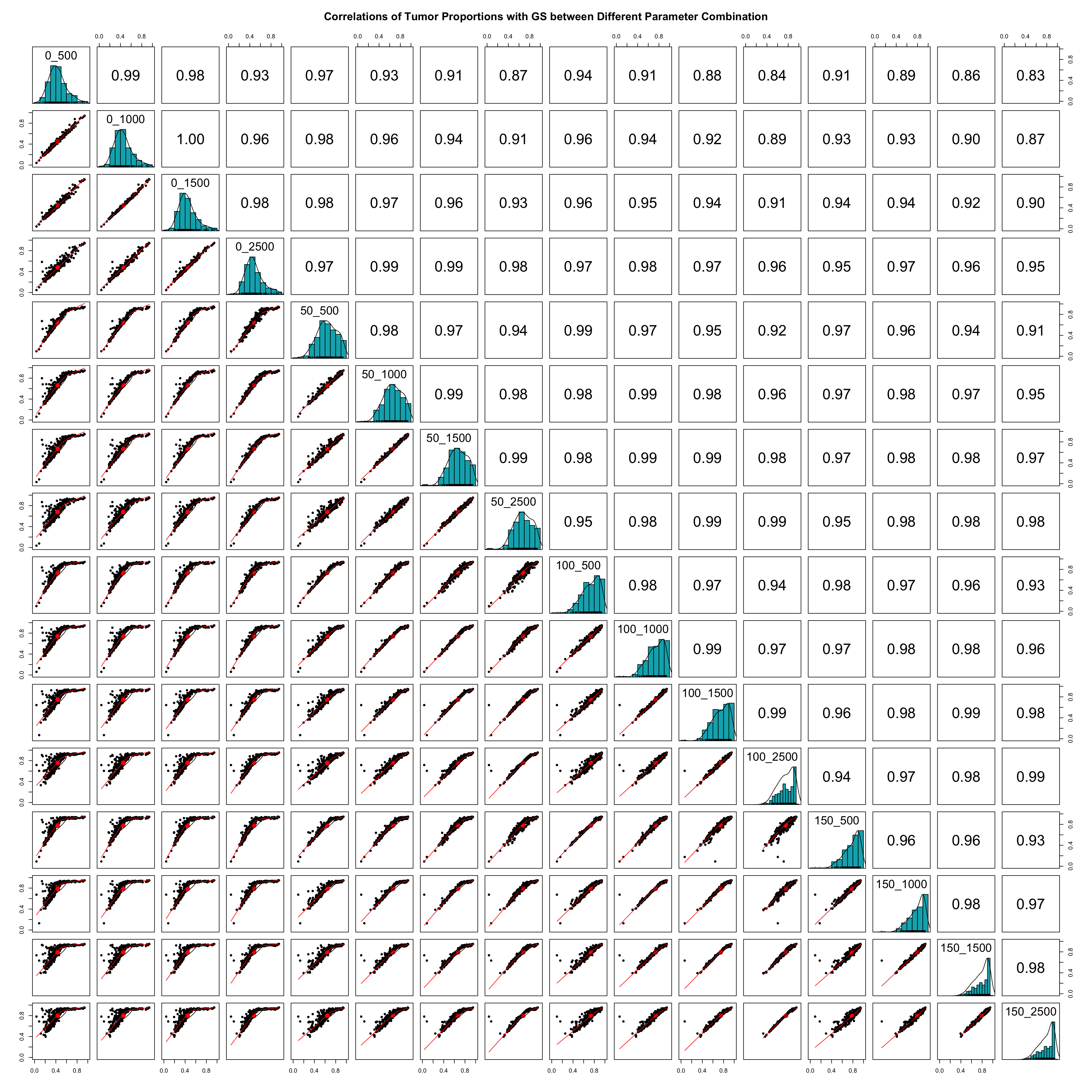
This step saves the deconvolution results (PiT) into a dataframe with columns named after the combination of the number of spike-ins and number of genes selected. Then one can calculate and plot the pairwise correlations of estimated tumor proportions across different parameter combinations as shown below.
pairs.panels(PiT_GS_PRAD,
            method = "spearman", # correlation method
            hist.col = "#00AFBB",
            density = TRUE,  # show density plots
            ellipses = TRUE, # show correlation ellipses
            main = 'Correlations of Tumor Proportions with GS between Different Parameter
            Combination',
            xlim = c(0,1),
            ylim = c(0,1))
Print out the average pairwise correlation of tumor proportions across different parameter combinations.
PiT_GS_PRAD <- as.data.frame(PiT_GS_PRAD)
Spearman_correlations <- list()

for(entry_1 in colnames(PiT_GS_PRAD)) {
  cor.values <- c()
  for (entry_2 in colnames(PiT_GS_PRAD)) {
    if (entry_1 == entry_2)
      next

    cor.values <- c(cor.values,
                    cor(PiT_GS_PRAD[, entry_1],
                    PiT_GS_PRAD[, entry_2],
                    method = "spearman"))
  }

  Spearman_correlations[[entry_1]] <- mean(cor.values)
}

Spearman_correlations <- unlist(Spearman_correlations)
Spearman_correlations <- data.frame(num.spikein_num.selected.gene=names(Spearman_correlations), mean.correlation=Spearman_correlations)

Spearman_correlations
The average correlation coefficient coefficients are listed below.
num.spikein_num.selected.gene   mean.correlation
0_500   0_500   0.8641319
0_1000  0_1000  0.9453534
0_1500  0_1500  0.9401355
0_2500  0_2500  0.9375468
5_500   5_500   0.9207604
5_1000  5_1000  0.9542926
5_1500  5_1500  0.9460006
5_2500  5_2500  0.8992011
10_500  10_500  0.9237941
10_1000 10_1000 0.9357266
10_1500 10_1500 0.9249267
10_2500 10_2500 0.9002124
We suggest selecting the optimal parameter combination that produces the highest average correlation of estimated tumor proportions. Additionally, consider the skewness of the PiT estimation distribution. Significant skewness may indicate biased estimation.
Based on these criteria, spike-ins = 5 and number of selected genes = 1000 are identified as the optimal parameter combination. Using these parameters, we can obtain the corresponding tumor proportions for each sample.
data.frame(sample.id=Tumor.id, PiT=PiT_GS_PRAD[['5_1000']])

sample.id               PiT
TCGA-2A-A8VL-01A    0.7596888
TCGA-2A-A8VO-01A    0.8421716
TCGA-2A-A8VT-01A    0.8662378
TCGA-2A-A8VV-01A    0.7616749
TCGA-2A-A8W1-01A    0.8291091
TCGA-2A-A8W3-01A    0.8159406
TCGA-CH-5737-01A    0.7314935
TCGA-CH-5738-01A    0.4614545
TCGA-CH-5739-01A    0.6349423
TCGA-CH-5740-01A    0.7095117
List the tumor specific expression
## Load the corresponding deconvolved gene expression
load("PRAD_demixt_GS_res_nspikesin_5_ngene.selected_1000.RData")
res$ExprT[1:5, 1:5]

      TCGA-2A-A8VL-01A TCGA-2A-A8VO-01A TCGA-2A-A8VT-01A TCGA-2A-A8VV-01A TCGA-2A-A8W1-01A
DPM1          1710.194         1466.484        1680.4562         1644.944         1812.600
FUCA2         3782.990         4083.382         961.0578         4165.612         1896.901
GCLC          2382.106         1826.957        1527.4895         1409.707         1913.784
LAS1L         3329.766         2758.414        3520.9410         2834.415         2530.621
ENPP4         2099.591         3123.365        3173.3516         2856.371         7413.330
Instead of selecting using the parameter combination with the highest correlation, one can also select the parameter combination that produces estimated tumor proportions that are most biologically meaningful.
The estimated tumor-specific proportions (PiT) can be used to calculate TmS. See our TmS tutorial.